by 3 Different Techniques
Polarization Resistance
We began with a simple LPR (Polarization Resistance) experiment. The results are shown to the right. Analysis of the data within 5 mV of Eoc gave the line shown in red. It corresponds to an Rp value of 687 ohm. Using the default beta values of 120 mV/decade yields a corrosion rate of 5.77 mpy in this electrolyte. This estimate can be refined if better estimates of the beta values are known. More about this shortly!
Electrochemical Impedance Spectroscopy
One way to check for the validity of a simple LPR experiment is to make an EIS measurement. The EIS measurement can also give an estimate of the solution resistance. A routine EIS measurement was performed at the Open Circuit Potential. The results of the EIS measurement are shown below. The red lines are the fit to the fairly simple model which is also shown. The inductor is needed to explain the high frequency phase shift. As in many systems, the double layer capacitance is best modeled by a constant phase element. The value of the polarization resistance, 674 +/- 13 ohm, agrees quite well with that from the LPR experiment! The uncompensated resistance (also known as the solution resistance) is quite small — less than 1 ohm.
 Electrochemical Frequency Modulation (EFM)
Finally, we ran the same sample using the EFM technique using frequencies of 20 mHz and 50 mHz. Both of these frequencies are on the low frequency plateau on the EIS plot, above. This is required by the EFM theory.
The results of the EFM analysis are shown to the right. The EFM technique has the advantage that the corrosion rate can be 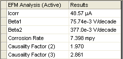 calculated without prior knowledge of the Tafel constants. The corrosion rate calculated from the EFM measurement is 7.4 mpy. The EFM measurement also gives an internal self-check in the form of the two “Causality Factors”. These two factors should have the values 2.0 and 3.0 if all of the conditions of EFM theory have been met. We see that our experiment meets the criteria!
The EFM corrosion rate (7.40 mpy) is in pretty good agreement with the rate (5.77) we calculated from the LPR measurement. However, the LPR calculation assumed that both betas were 120 mV/decade. Now that we have estimates for the Tafel constants from the EFM measurement, we can recalculate the LPR corrosion rate. The table, below, summarizes the data from all three experiments. The agreement between the three non-destructive techniques is excellent!