
 One guideline that I have heard recommended (although I cannot give a reference for it) is that data over a decade range of frequency is required to support each circuit component.
All curve-fitting software should report some measure of the “goodness of fit.” Often this is the chi-squared parameter ( X2 ) or a value related to it. Boukamp makes the recommendation that the value of X2 should decrease by tenfold if a new circuit element is introduced into the circuit model. The tenfold decrease provides the justification for including the new circuit element. If the inclusion of an additional circuit element does not substantially improve the goodness-of-fit (as evidenced by the decrease in the X2 value), then based on Occam’s Razor, you should keep the simpler model, or continue your search for an improved one.
The old joke about the ability to “fit an elephant” if you use enough parameters is all too true with impedance data. Each component added to the model should have a physical explanation. Adding components only because they make the fit look better (smaller X2) without a physical interpretation is the equivalent to “fitting an elephant.”
What is X2?
When we hear about “least squares,” it is X2 that is being minimized. What is it? And how can I relate its value to a “goodness-of-fit” that I can understand?
If we are trying to fit some data, y, to a known function, f(x), we can write chi-squared as (See Numerical Recipes in C, Chapter. 15)
(1)
In this equation, is the standard deviation of measurement i, which may be different for each point measured. The problem with X² as written is that its value depends on the number of points used! Simply duplicating all of your data points doubles the value of X²! Consequently, I prefer to look at X²/(n-m), where m is the number of adjustable parameters in the fit, and (n-m) is the number of degrees of freedom. If the estimates for are reasonable, then X²/(n-m) should approximate unity, regardless of the number of data points, and different data sets are easily compared.
In many electrochemical experiments, the current varies widely over the course of the experiment, and it is measured by a potentiostat that is used in the autoranged mode. This is generally true of a Tafel experiment in a corrosion application, or in an EIS measurement over several decades of frequency. Many of the instrumental sources of noise (e.g., quantization noise at the ADC, or amplifier noise in the signal chain) lead to errors which are (approximately) a fixed fraction, , of the full scale current. Because the autoranging algorithm strives to keep the measured current (yi) close to the full scale current, we may write: . Further, we see that with this assumption, weighting each of the points by yi allows us to recast equation (1) as
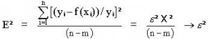
(2)
Minimizing E2 is the same as minimizing X2 with this weighting assumption. However, taking the square root of E2 gives the relative error in the measured current (i.e., ! ) That is a number most of us can understand! A value of E2 of 1e-4 translates to an average 1% error in the measured y values. [ sqrt( E2 ) = sqrt( 1E-4 ) = 0.01 ==> 1% ]