
This application note presents an introduction to Electrochemical Impedance Spectroscopy (EIS) theory and has been kept as free from mathematics and electrical theory as possible. If you still find the material presented here difficult to understand, don’t stop reading. You will get useful information from this application note, even if you don’t follow all of the discussions.
Four major topics are covered in this Application Note.
- AC Circuit Theory and Representation of Complex Impedance Values
- Physical Electrochemistry and Circuit Elements
- Common Equivalent Circuit Models
- Extracting Model Parameters from Impedance Data
No prior knowledge of electrical circuit theory or electrochemistry is assumed. Each topic starts out at a quite elementary level, then proceeds to cover more advanced material.
AC Circuit Theory and Representation of Complex Impedance Values
Impedance Definition: Concept of Complex Impedance

(1)
Almost everyone knows about the concept of electrical resistance. It is the ability of a circuit element to resist the flow of electrical current. Ohm’s law (Equation 1) defines resistance in terms of the ratio between voltage, E, and current, I.
While this is a well known relationship, its use is limited to only one circuit element — the ideal resistor. An ideal resistor has several simplifying properties:
- It follows Ohm’s Law at all current and voltage levels.
- Its resistance value is independent of frequency. AC current and voltage signals though a resistor are in phase with each other.
However, the real world contains circuit elements that exhibit much more complex behavior. These elements force us to abandon the simple concept of resistance, and in its place we use impedance, a more general circuit parameter. Like resistance, impedance is a measure of the ability of a circuit to resist the flow of electrical current, but unlike resistance, it is not limited by the simplifying properties listed above.
Electrochemical impedance is usually measured by applying an AC potential to an electrochemical cell and then measuring the current through the cell. Assume that we apply a sinusoidal potential excitation. The response to this potential is an AC current signal. This current signal can be analyzed as a sum of sinusoidal functions (a Fourier series).
Electrochemical impedance is normally measured using a small excitation signal. This is done so that the cell’s response is pseudo-linear. In a linear (or pseudo-linear) system, the current response to a sinusoidal potential will be a sinusoid at the same frequency but shifted in phase (see Figure 1). Linearity is described in more detail in the following section.
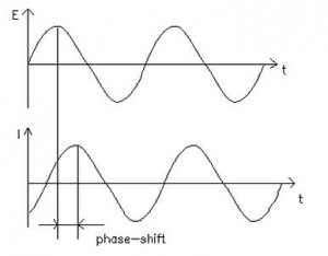
Figure 1. Sinusoidal Current Response in a Linear System
The excitation signal, expressed as a function of time, has the form
(2)
where Et is the potential at time t, E0 is the amplitude of the signal, and ω is the radial frequency. The relationship between radial frequency ω (expressed in radians/second) and frequency f (expressed in hertz) is:
(3)
In a linear system, the response signal, It, is shifted in phase (Φ) and has a different amplitude than I0.
(4)
An expression analogous to Ohm’s Law allows us to calculate the impedance of the system as:
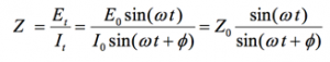
(5)
The impedance is therefore expressed in terms of a magnitude, Zo, and a phase shift, Φ.
If we plot the applied sinusoidal signal E(t) on the X-axis of a graph and the sinusoidal response signal I(t) on the Y-axis, the result is an oval (see Figure 2). This oval is known as a “Lissajous Figure”. Analysis of Lissajous Figures on oscilloscope screens was the accepted method of impedance measurement prior to the availability of modern EIS instrumentation.
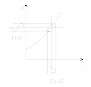
Figure 2. Origin of Lissajous Figure
With Eulers relationship,
(6)
it is possible to express the impedance as a complex function. The potential is described as,
(7)
and the current response as,
(8)
The impedance is then represented as a complex number,
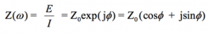
(9)
Data Presentation
Read the complete Basics of Electrochemical Impedance Spectroscopy application notedownload this note in PDF format.