CPE in parallel with a resistance

The Constant Phase Element (CPE)

What is a Constant Phase Element?

The Constant Phase Element (CPE) is a non-intuitive circuit element that was discovered (or invented) while looking at the response of real-world systems. In some systems the Nyquist plot (also called the Cole-Cole plot or Complex Impedance Plane plot) was expected to be a semicircle with the center on the x-axis. However, the observed plot was indeed the arc of a circle, but with the center some distance below the x-axis.
These depressed semicircles have been explained by a number of phenomena, depending on the nature of the system being investigated. However, the common thread among these explanations is that some property of the system is not homogeneous or that there is some distribution (dispersion) of the value of some physical property of the system.

CPE equations

Mathematically, a CPE’s impedance is given by

1 / Z = Y = Q° ( j omega )n

where Q° has the numerical value of the admittance (1/ |Z|) at omega =1 rad/s. The units of Q° are S•sn (ref 1).
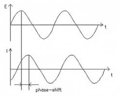
A consequence of this simple equation is that the phase angle of the CPE impedance is independent of the frequency and has a value of -(90*n) degrees. This gives the CPE its name.

When n=1, this is the same equation as that for the impedance of a capacitor, where Q° =C.

1 / Z = Y = j omega Q° = j omega C

When n is close to 1.0, the CPE resembles a capacitor, but the phase angle is not 90°. It is constant and somewhat less than 90° at all frequencies. In some cases, the ‘true’ capacitance can be calculated from Q° and n
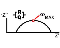
The Nyquist (Complex Impedance Plane) Plot of a CPE is a simple one. For a solitary CPE (symbolized here by Q), it is just a straight line which makes an angle of (n*90°) with the x-axis as shown in pink in the Figure. The plot for a resistor (symbolized by R) in parallel with a CPE is shown in green. In this case the center of the semicircle is depressed by an angle of (1-n)*90°

What Causes a CPE?

[…]

Electrochemistry Impedance Spectroscopy Basics

Basics of Electrochemical Impedance Spectroscopy

This application note presents an introduction to Electrochemical Impedance Spectroscopy (EIS) theory and has been kept as free from mathematics and electrical theory as possible. If you still find the material presented here difficult to understand, don’t stop reading. You will get useful information from this application note, even if you don’t follow all of the discussions.

Four major topics are covered in this Application Note.

  • AC Circuit Theory and Representation of Complex Impedance Values
  • Physical Electrochemistry and Circuit Elements
  • Common Equivalent Circuit Models
  • Extracting Model Parameters from Impedance Data

No prior knowledge of electrical circuit theory or electrochemistry is assumed. Each topic starts out at a quite elementary level, then proceeds to cover more advanced material.

AC Circuit Theory and Representation of Complex Impedance Values

Impedance Definition: Concept of Complex Impedance

concept of electrical resistance

(1)

Almost everyone knows about the concept of electrical resistance. It is the ability of a circuit element to resist the flow of electrical current. Ohm’s law (Equation 1) defines resistance in terms of the ratio between voltage, E, and current, I.

While this is a well known relationship, its use is limited to only one circuit element — the ideal resistor. An ideal resistor has several simplifying properties:

  • It follows Ohm’s Law at all current and voltage levels.
  • Its resistance value is independent of frequency. AC current and voltage signals though a resistor are in phase with each other.

[…]

This website uses cookies to ensure you get the best experience on our website. More information

The cookie settings on this website are set to "allow cookies" to give you the best browsing experience possible. If you continue to use this website without changing your cookie settings or you click "Accept" below then you are consenting to this. Please review our Privacy Policy

Close